from google.colab import drive
drive.mount('/content/drive')

# Libraries to help with reading and manipulating data
import numpy as np
import pandas as pd

# Libraries to help with data visualization
import matplotlib.pyplot as plt
import seaborn as sns

# Command to tell Python to actually display the graphs
%matplotlib inline

df = pd.read_csv('Automobile (1).csv')
# df = pd.read_csv('/location on your computer/Automobile (1).csv')

df.head()

Output:

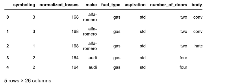
df.shape

Output: (201, 26)
• The data has 201 rows and 26 columns.

df.info()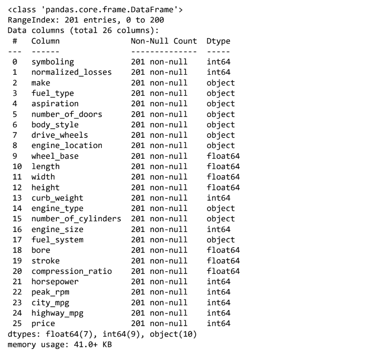

• There are attributes of different types (int, float, object) in the data.

df.describe(include='all').T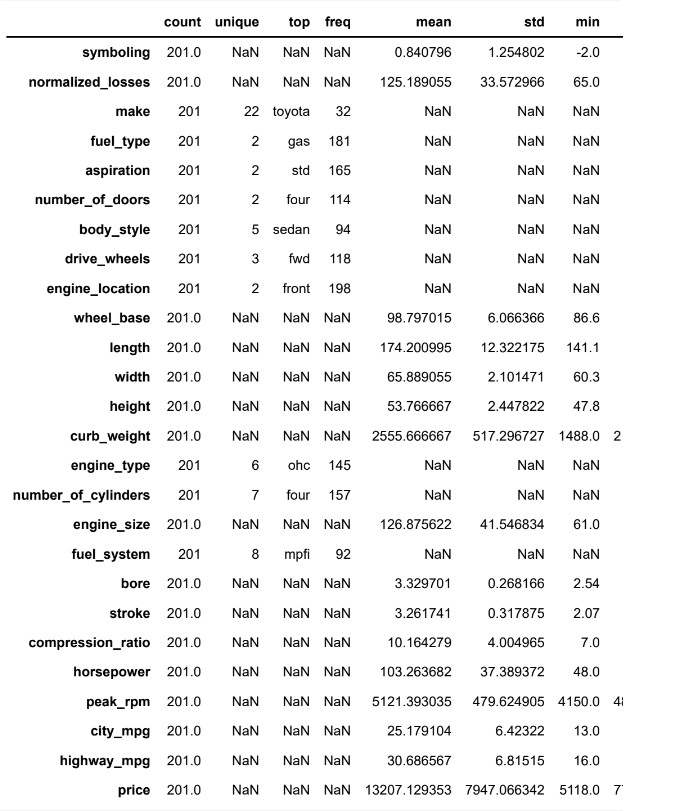

• The car price ranges from 5118 to 45400 units.
• The car weight ranges from 1488 to 4066 units.
• The most common car make in the data is of Toyota.

Histogram

• A histogram is a univariate plot which helps us understand the distribution of a continuous numerical variable.

• It breaks the range of the continuous variables into a intervals of equal length and then counts the number of observations in each interval.

• We will use the histplot() function of seaborn to create histograms.

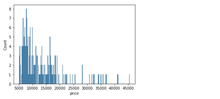
sns.histplot(data=df, x='price')

Output: <AxesSubplot:xlabel='price', ylabel='Count'>

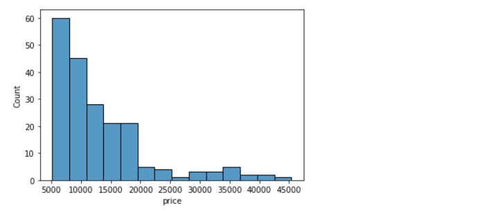
Let's see how we can customize a histogram.

plt.title('Histogram:Price')
plt.xlim(3000,50000)
plt.ylim(0,70)
plt.xlabel('Price of cars')
plt.ylabel('Frequency')
sns.histplot(data=df, x='price',color='orange');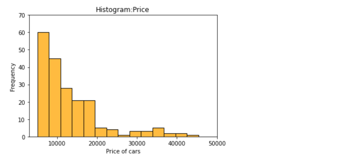

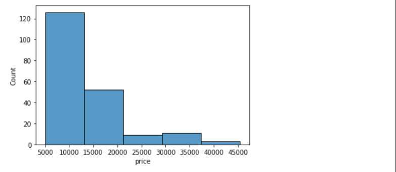
We can specify the number of intervals (or groups or bins) to create by setting the bins parameter.

• If not specified it is passed to numpy.histogram_bin_edges()(https://numpy.org/doc/stable/reference/generated/numpy.histogram_bin_edges.html#numpy.histogram_bin_edges

sns.histplot(data=df, x='price', bins=5)

Output: <AxesSubplot:xlabel='price', ylabel='Count'>

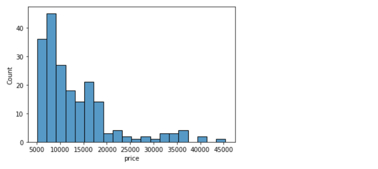
sns.histplot(data=df, x='price', bins=20)

Output: <AxesSubplot:xlabel='price', ylabel='Count'>

If we want to specify the width of the intervals (or groups or bins), we can use binwidth parameter.

sns.histplot(data=df, x='price', binwidth=20)

Output: <AxesSubplot:xlabel='price', ylabel='Count'>

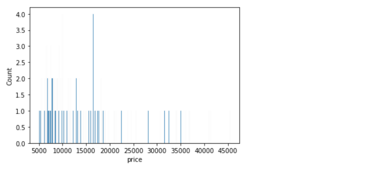
sns.histplot(data=df, x='price', binwidth=200)

Output: <AxesSubplot:xlabel='price', ylabel='Count'>

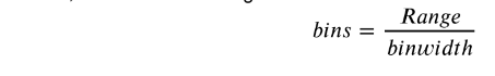
How to find the optimal number of bins: Rule of thumb

• We calculate the bin-width first, using the following formula:

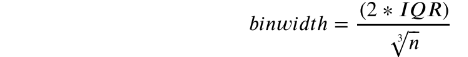
where n = number of rows the dataset

• Then, we obtain bins using the calculated bin-width.

In addition to the bars, we can also add a density estimate by setting the kde parameter to True.

• Kernel Density Estimation, or KDE, visualizes the distribution of data over a continuous interval.
The conventional scale for KDE is: Total frequency of each bin × Probability

sns.histplot(data=df, x='price', kde=True);

sns.histplot(data=df, x='price', bins=700, kde=True);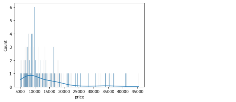

Clearly, if we increase the number of bins, it reduces the frequency count in each group (bin). Since the scale of KDE depends on the total frequency of each bin (group), the above code gives us a flattened KDE plot.

Let's check out the histograms for a few more attributes in the data.

sns.histplot(data=df, x='curb_weight', kde=True);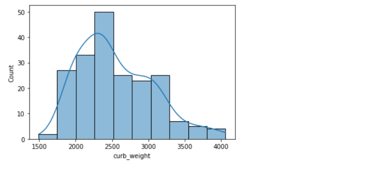

• A histogram is said to be symmetric if the left-hand and right-hand sides resemble mirror images of each other when the histogram is cut down the middle.

sns.histplot(data=df, x='horsepower', kde=True);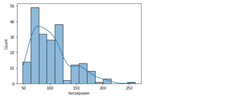

• The tallest clusters of bars, i.e., peaks, in a histogram represent the modes of the data.
• A histogram skewed to the right has a large number of occurrences on the left side of the plot and a few on the right side of the plot.
• Similarly, a histogram skewed to the left has a large number of occurrences on the right side of the plot and few on the left side of the plot.

Histograms are intuitive but it is hardly a good choice when we want to compare the distributions of several groups. For example,

sns.histplot(data=df, x='price', hue='body_style', kde=True);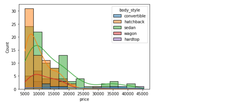

It might be better to use subplots!

g = sns.FacetGrid(df, col="body_style")
g.map(sns.histplot, "price");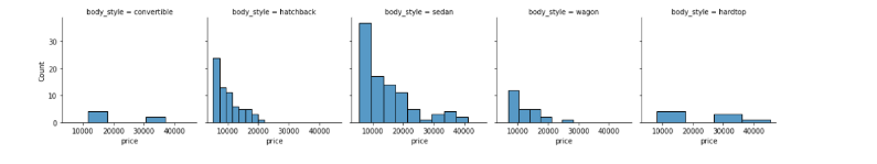

In such cases, we can use boxplots. Boxplots, or box-and-whiskers plots, are an excellent way to visualize differences among groups.

Boxplot

• A boxplot, or a box-and-whisker plot, shows the distribution of numerical data and skewness through displaying the data quartiles
• It is also called a five-number summary plot, where the five-number summary includes the minimum value, first quartile, median, third quartile, and the maximum value.
• The boxplot() function of seaborn can be used to create a boxplot.

To get this project in deatils, Download Here